Validation

The two primary approaches to validating experimental data included in DearEIS are linear Kramers-Kronig testing and Z-HIT analysis. The former is a widely adopted approach based on attempting to fit a specific type of equivalent circuit, which is known a priori to be Kramers-Kronig transformable. The latter approach reconstructs the modulus data from the (typically) more stable phase data, which can reveal issues such as drift at low frequencies due to time invariant behavior exhibited by the measured system.

Kramers-Kronig testing

Data validation based on linear Kramers-Kronig testing can be performed in the Kramers-Kronig tab (Fig. 10) which contains the following:

• various settings that determine how the Kramers-Kronig test is performed

• combo boxes that can be used to choose the active data set and the active test result

• a table of statistics related to the active test result

• a table of settings that were used to obtain the active result

• different plots

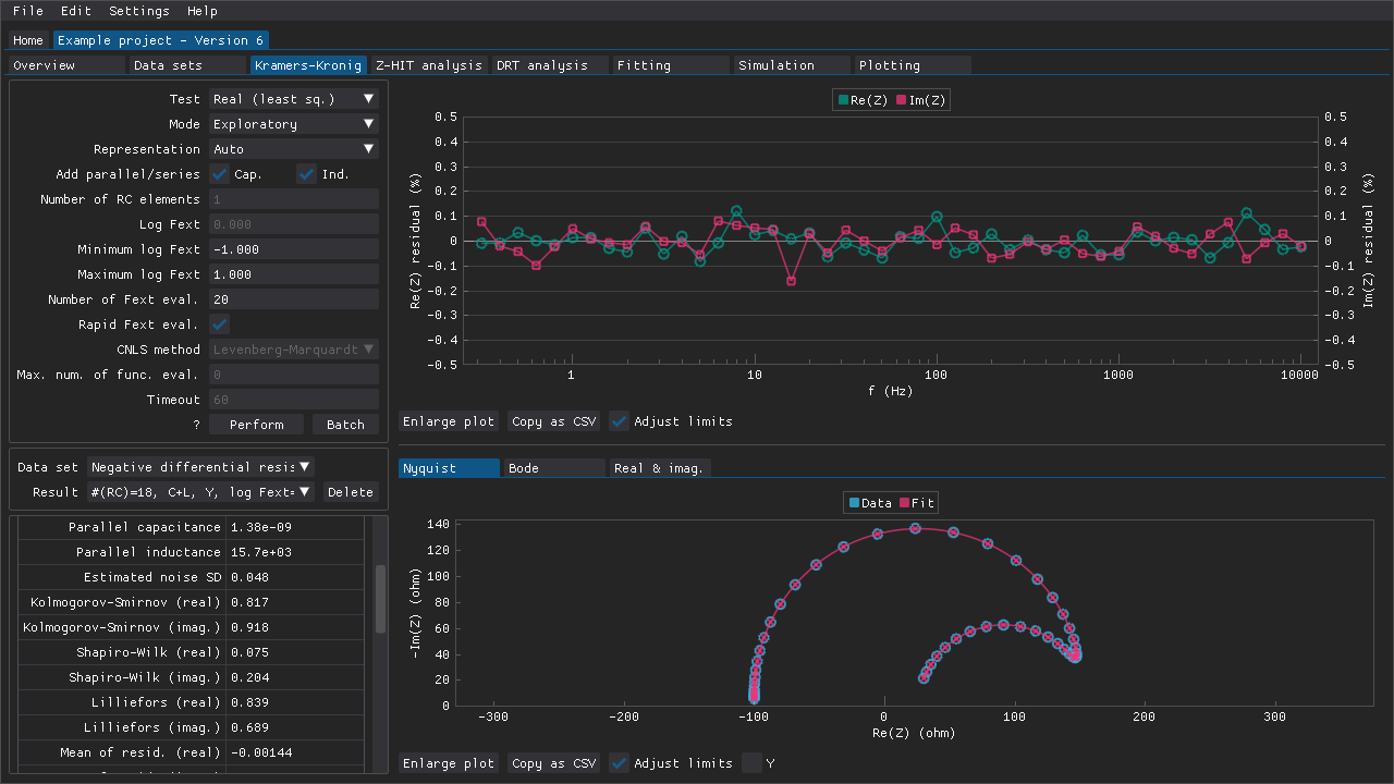
Fig. 10 A Kramers-Kronig test result for an impedance spectrum with a negative differential resistance.

The three variants of the linear Kramers-Kronig test (complex, real, and imaginary) described by Boukamp (1995) have been included. These have been implemented using either least squares fitting or matrix inversion. There is also an implementation that uses complex non-linear least squares fitting. These tests can be performed with a fixed number of time constants (i.e., RC elements), \(N_\tau\), using the Manual mode. However, it is recommended that \(N_\tau\) is determined automatically using one or more methods of the following methods by using either the Auto or the Exploratory mode.

Table 2 Methods for suggesting the optimum number of time constants (i.e., the number of parallel/series RC elements).

Method	Reference
1: \({\rm \mu}\)-criterion	Schönleber et al. (2014)
2: norm of fitted variables	Plank et al. (2022)
3: norm of curvatures	Plank et al. (2022)
4: number of sign changes among curvatures	Plank et al. (2022)
5: mean distance between sign changes among curvatures	Yrjänä and Bobacka (2024)
6: apex of \(\log{\Sigma_{k=1}^{N_\tau} |\tau_k / R_k|}\) (or \(\log{\Sigma_{k=1}^{N_\tau} |\tau_k / C_k|}\)) versus \(N_\tau\)	Yrjänä and Bobacka (2024)

The intermediate results of these methods can be inspected in the Exploratory mode as a means of detecting and dealing with issues such as false negatives.

Note

A custom combination of methods 3, 4, and 5 is used by default. However, a specific method or combination of methods can be chosen via the window that shows up when using the Exploratory mode or via the Settings > Defaults window.

In addition to \(N_\tau\), the range of time constants can and should also be optimized. The range of time constants are by default defined by the reciprocals of the maximum and minimum frequencies of the impedance spectrum. However, the limits can be adjusted by an extension factor, \(F_{\rm ext}\), which is initially set to \(\log{F_{ext}} = 0\) in terms of the settings provided in DearEIS. The optimal range of time constants may be wider (\(\log{F_{ext}} > 0\)) or narrower (\(\log{F_{ext}} < 0\)) than the default range. There are settings for the limits to use when optimizing \(\log{F_{\rm ext}}\) and the number of evaluations to perform. A specific \(\log{F_{\rm ext}}\) can also be used directly by setting the number of evaluations to zero.

Some immittance spectra may need to be validated using based on their admittance representations rather than their impedance representations. It is therefore recommended that the Representation setting is set to Auto, which results in both the impedance and the admittance representation being tested.

Note

If you only wish to validate the impedance representation of the immittance data, then see Adding parallel impedances for information about how to process impedance data that include, e.g., negative differential resistances before attempting to validate the data.

The test results are presented in the form of a table of statistics (e.g., \(\chi^2_{ps.}\) which indicates the quality of the fit) and different plots such as one of the relative residuals of the fit.

Exploratory mode

If the Exploratory mode is used, then the intermediate results of the linear Kramers-Kronig test and the various methods for suggesting the optimal number of RC elements are presented in a window that pops up. The main advantages of using the Exploratory mode over the Auto mode are that one can:

• evaluate how \(\chi^2_{ps.}\) behaves as a function of \(\log{F_{\rm ext}}\) and \(N_\tau\), and how the values used by the different methods for suggesting the optimal \(N_\tau\) behave

• manually adjust, e.g., the representation, \(\log{F_{\rm ext}}\), and/or \(N_\tau\)

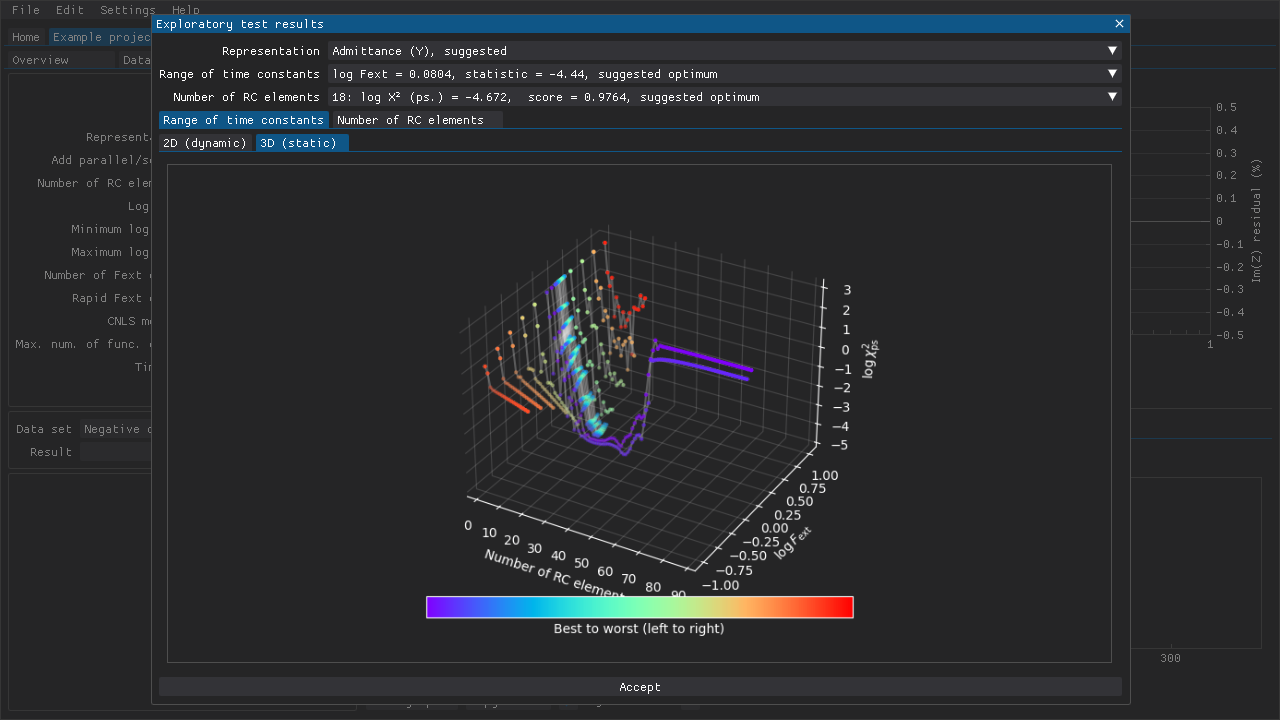
Fig. 11 The extension or contraction of the range of time constants can be evaluated using a 3D plot as shown here. Rapid (i.e. partial) evaluations of different \(\log{F_{\rm ext}}\) values have been used here. The full range of \(N_\tau\) have only been evaluated with the initial \(\log{F_{ext}} = 0\) and the optimal \(\log{F_{ext}} = -0.151\).

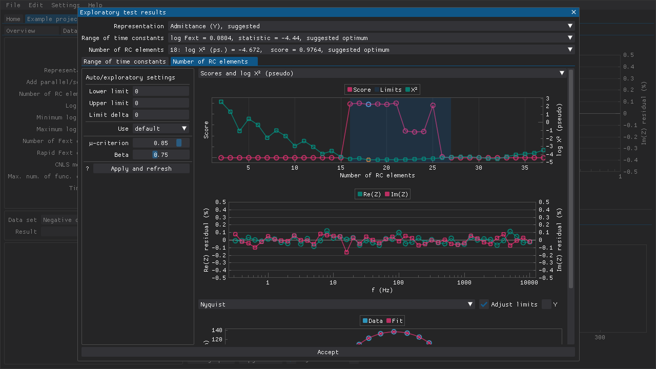
Fig. 12 The settings for suggesting the optimal number of RC elements can be adjusted. By default, the lower and upper limits are suggested automatically, and then a combination of methods 3, 4, and 5 are used to suggest the number of RC elements. Various plots can be viewed to evaluate the results.

References:

• Boukamp, B.A., 1995, J. Electrochem. Soc., 142, 1885-1894

• Schönleber, M., Klotz, D., and Ivers-Tiffée, E., 2014, Electrochim. Acta, 131, 20-27

• Plank, C., Rüther, T., and Danzer, M.A., 2022, 2022 International Workshop on Impedance Spectroscopy (IWIS), pp. 1–6

• Yrjänä, V. and Bobacka, J., 2024, Electrochim. Acta, 504, 144951

Z-HIT analysis

Data validation using the Z-HIT algorithm can be performed in the Z-HIT analysis tab (Fig. 13) that contains the following:

• the various settings that determine how the Z-HIT analysis is performed

• combo boxes that can be used to choose the active data set and the active analysis result

• a table of statistics related to the active analysis result

• a table of the settings that were used to obtain the active result

• different plots

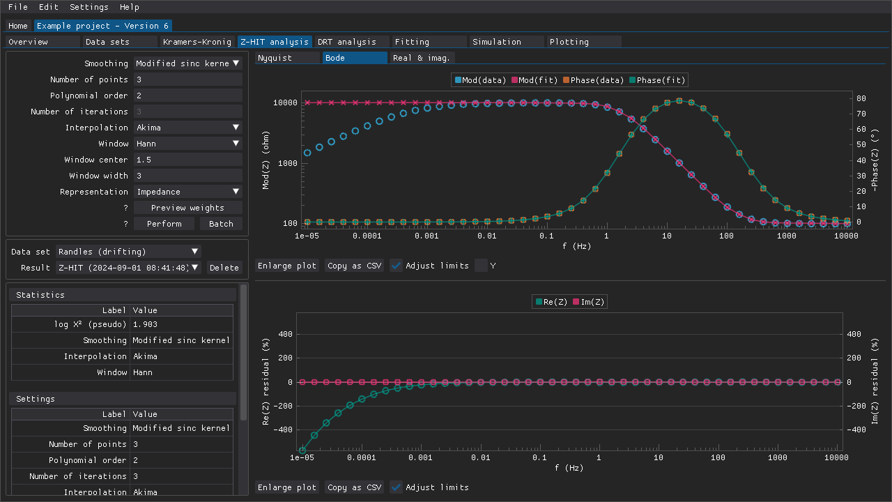
Fig. 13 The modulus data that is plotted in the upper plot has been reconstructed (red line) based on the phase data (orange markers and green line) of some example data that exhibits drift at low frequencies (blue markers).

The Z-HIT algorithm was first described by Ehm et al. (2000) and provides a means of validating recorded impedance spectra using a modified logarithmic Hilbert transformation. The phase data is typically smoothed before it is interpolated using a spline, and then it is integrated and derivated to reconstruct the modulus data. The final step is an adjustment of the offset of the reconstructed modulus data by fitting to a subset of the experimental data that is unaffected by, e.g., drift. This subset of data points is typically in the range of 1 Hz to 1000 Hz.

Note

The modulus data is not reconstructed perfectly. There are often minor deviations even with ideal data.

DearEIS offers a few options for smoothing algorithm and interpolation spline, and several different window functions for the weights to use during offset adjustment. The weights can also be previewed in a window (Fig. 14) that is accessible via the Preview weights button that is located below the section for settings. This window can help with selecting a window function and appropriate parameters for it.

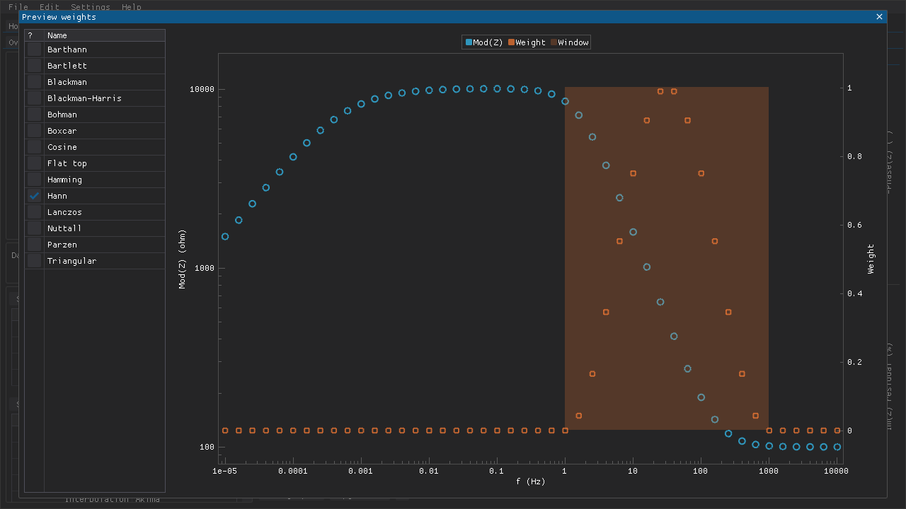
Fig. 14 It is possible to preview the weights that could be applied when fitting the approximated modulus data to the experimental modulus data. The shaded region shows the position of the window function while the orange markers show the weight (from 0.0 to 1.0) that could be applied.

The results are presented in the form of a table of statistics and different plots.

References:

• Ehm, W., Göhr, H., Kaus, R., Röseler, B., and Schiller, C.A., 2000, Acta Chimica Hungarica, 137 (2-3), 145-157.

• Ehm, W., Kaus, R., Schiller, C.A., and Strunz, W., 2001, in “New Trends in Electrochemical Impedance Spectroscopy and Electrochemical Noise Analysis”.

• Schiller, C.A., Richter, F., Gülzow, E., and Wagner, N., 2001, 3, 374-378

Applying old settings and masks

The settings that were used to perform the active test result are also presented as a table and these settings can be applied by pressing the Apply settings button.

The mask that was applied to the data set when the test was performed can be applied by pressing the Apply mask button. If the mask that is applied to the data set has changed since an earlier analysis was performed, then that will be indicated clearly above the statistics table.

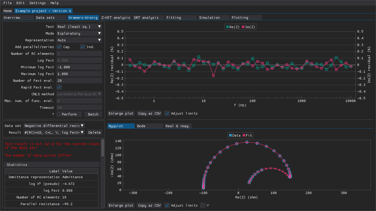
Fig. 15 An example of the warning (red text on the left-hand side) that could be shown if, e.g., the mask applied to a data set has been changed after an analysis has been performed. In this case, several points of the high-frequency semi-circle in the Nyquist plot have been omitted.

These features make it easy to restore old settings/masks in case, e.g., DearEIS has been closed and relaunched, or after trying out different settings.