Distribution of relaxation times analysis

Performing analyses

The distribution of relaxation times (DRT) can be calculated using multiple different approaches (see the corresponding publications for details):

This type of analysis can be used, e.g., as an aid when developing equivalent circuits by revealing the number of time constants. The peak shapes (e.g., symmetry and sharpness) can also help with identifying circuit elements that could be suitable.

DRT calculations can be performed in the DRT analysis tab (Fig. 16):

the various settings that determine how the DRT calculations are performed
combo boxes that can be used to choose the active data set and the active result, and a button for deleting the active result
a table of statistics related to the active result
a table of the settings that were used to obtain the active result

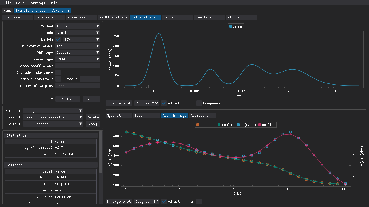
The DRT analysis tab of a project — Fig. 16 An example of a result obtained with the noisy data set and the TR-RBF method.

The results are presented in the form of one or more tables (e.g., statistics, scores), a plot of gamma versus time constant, and other plots. Some results can be copied to the clipboard in different plain-text formats via the Output combo box and the Copy button.

It was mentioned in the Processing data subchapter that some forms of analysis can be sensitive to the omission of a data point. Below are some examples of this. The overlay plots shown below are created using the Plotting tab (more information about that can be found in the Plotting subchapter).

Fig. 17 Three overlaid DRT spectra that were obtained with the TR-RBF method using the same settings: with outlier (original), without outlier (omitted), and with the outlier replaced (interpolated). The presence of the outlier clearly has a significant effect on peak positions in the range above 0.001 s. However, omitting the outlier resulted in additional peaks appearing within the 0.01 to 0.1 s range.

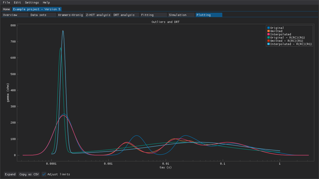
Six overlaid DRT spectra — Fig. 18 Additional DRT spectra, which were obtained by fitting **R(RC)(RQ)** circuits and calculating the DRT using the m(RQ)fit method, overlaid on top of Fig. 17. The presence of the outlier has shifted the peaks toward lower time constants (original). The m(RQ)fit method is less sensitive to the omission of the outlier as can be seen from the two DRT spectra (omitted and interpolated) that are almost identical. The two latter spectra also have, e.g., their left-most peaks in the correct position of approximately 0.00016 s which is the expected value based on the known resistance and capacitance values (200 \(\Omega\) and 0.8 \(\mathrm{\mu F}\), respectively) of the circuit that was used to generate the data sets.

One can see based on Fig. 18 that different DRT methods can produce very different results, but the settings and amount of noise in the data also have a significant effect as can be seen in Fig. 19.

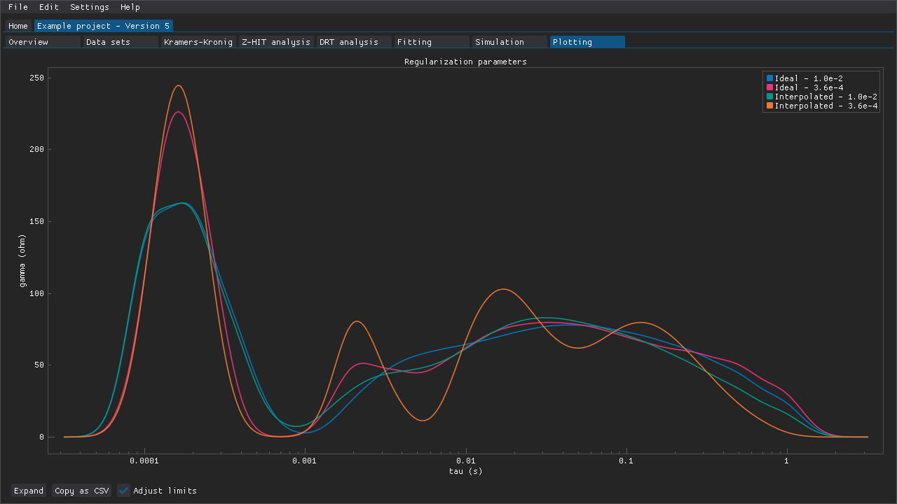
Four overlaid DRT spectra — Fig. 19 In this example two DRT spectra are shown for each of the data sets: ideal (no noise) and interpolated (noisy with the outlier replaced). The DRT spectra have been obtained using the TR-RBF method with otherwise identical settings apart from the regularization parameters, \(\lambda\), that are indicated in the labels found in the plot legend.

References:

Applying old settings and masks

The settings that were used to perform the active analysis result are also presented as a table and these settings can be applied by pressing the Apply settings button.

The mask that was applied to the data set when the analysis was performed can be applied by pressing the Apply mask button. If the mask that is applied to the data set has changed since an earlier analysis was performed, then that will be indicated clearly above the statistics table.

These features make it easy to restore old settings/masks in case, e.g., DearEIS has been closed and relaunched, or after trying out different settings.

References:

Boukamp, B.A. and Rolle, A, 2017, Solid State Ionics, 302, 12-18
Ciucci, F. and Chen, C., 2015, Electrochim. Acta, 167, 439-454
Effat, M. B. and Ciucci, F., 2017, Electrochim. Acta, 247, 1117-1129
Liu, J., Wan, T. H., and Ciucci, F., 2020, Electrochim. Acta, 357, 136864
Wan, T. H., Saccoccio, M., Chen, C., and Ciucci, F., 2015, Electrochim. Acta, 184, 483-499