Processing data

The Data sets tab

Multiple impedance spectra (or data sets) can be loaded and processed in the Data sets tab (Fig. 3) that contains the following:

• Data set combo for switching between data sets that have been loaded via the Load button.

• Label input for modifying the label assigned to the current data set.

• Path input for modifying the file path assigned to the current data set.

• Process button for opening a popup window with buttons for accessing features that enable further processing of the current data set.

• A table of data points with the ability to mask (i.e., hide/exclude) individual points (e.g., outliers).

• Toggle points button for (un)masking multiple points at once.

• Copy mask button for copying a mask from another data set and applying it to the current data set.

• Enlarge/show plot button for viewing a larger version of the current plot type.

• Adjust limits checkbox for enabling/disabling automatic adjustment of plot limits when switching between data sets.

• Plot type combo for switching between plot types. This is primarily for use when the program window is so narrow that the plots are hidden in order to keep the table of data points from becoming to narrow.

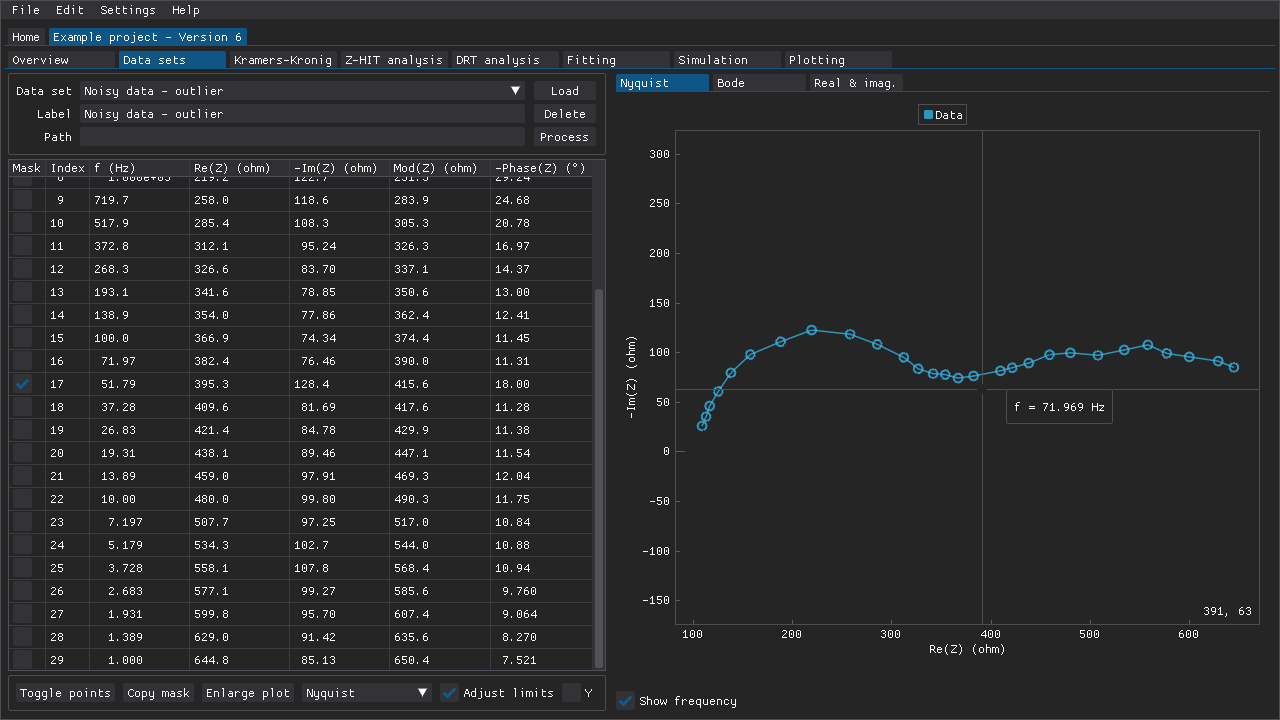
Fig. 3 The data point around 50 Hz has been omitted from this rather noisy data set as an outlier.

Supported file formats

Several different file formats are supported:

• BioLogic: .mpt

• Eco Chemie: .dfr

• Gamry: .dta

• Ivium: .idf and .ids

• Spreadsheets: .xlsx and .ods

• Plain-text character-separated values (CSV): .csv and .txt

Additional file formats may be supported in the future.

Not all CSV files and spreadsheets are necessarily supported as-is but the parsing of those types of files should be quite flexible in terms of, e.g., the characters that are used as separators. The parsers expect to find at least a column with frequencies (Hz) and columns for either the real and imaginary parts of the impedance (\(\Omega\)), or the absolute magnitude (\(\Omega\)) and the phase angle/shift (degrees). The supported column headers are:

• frequency: frequency, freq, or f

• real: z', z_re, zre, real, or re

• imaginary: z", z'', z_im, zim, imaginary, imag, or im

• magnitude: |z|, z, magnitude, modulus, mag, or mod

• phase: phase, phz, or phi

The identification of column headers is case insensitive (i.e., Zre and zre are considered to be the same). The sign of the imaginary part of the impedance and/or the phase angle/shift may be negative, but then that has to be indicated in the column header with a - prefix (e.g., -Zim or -phase).

Masking data points

Masks can be applied to hide data points in several ways and masked data points are excluded from plots and analyses. This feature can be used to get rid of outliers or to analyze a fragment of a data set. Individual data points can be masked via the checkboxes along the left-hand side of the table of data points (Fig. 3). Ranges of data points can be toggled via the window that is accessible via the Toggle points button below the table of data points. This can be used to, e.g., quickly mask multiple points or to remove the mask from all points (Fig. 4). Middle-mouse clicking and dragging a region in a plot in that window can also be used to choose the points to toggle.

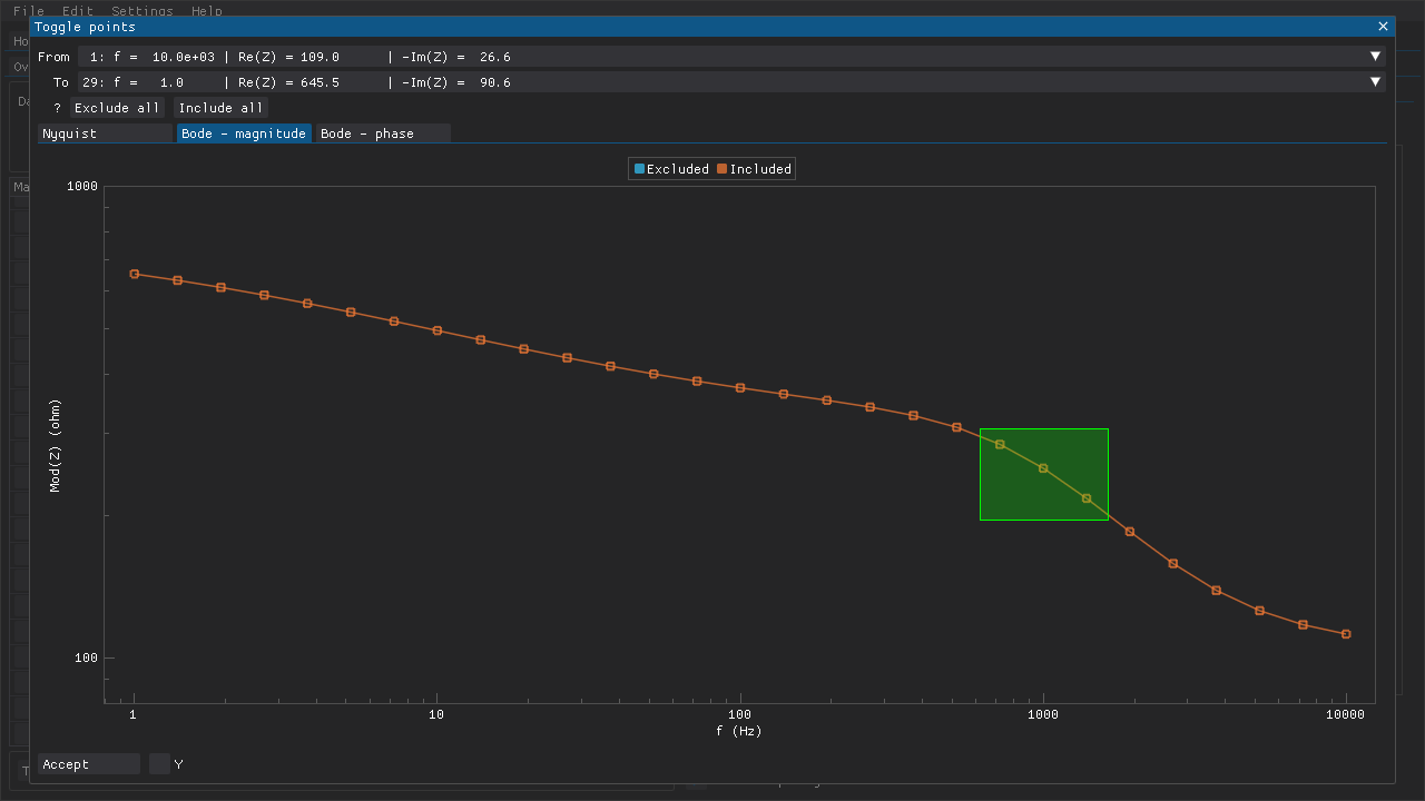
Fig. 4 The Toggle points can be used to (un)mask multiple data points in several ways. A preview of what the current data set would look like with the new mask is also included. Here a region has been highlighted in one of the plots by holding down the middle-mouse button and dragging. All of the points are included, which means that the points within the highlighted region will be toggled (i.e., excluded) when the Accept button is clicked.

If multiple data sets will need to have the same (or very similar) masks, then the Copy mask window can be used to copy the applied mask from another data set to the current data set (Fig. 5).

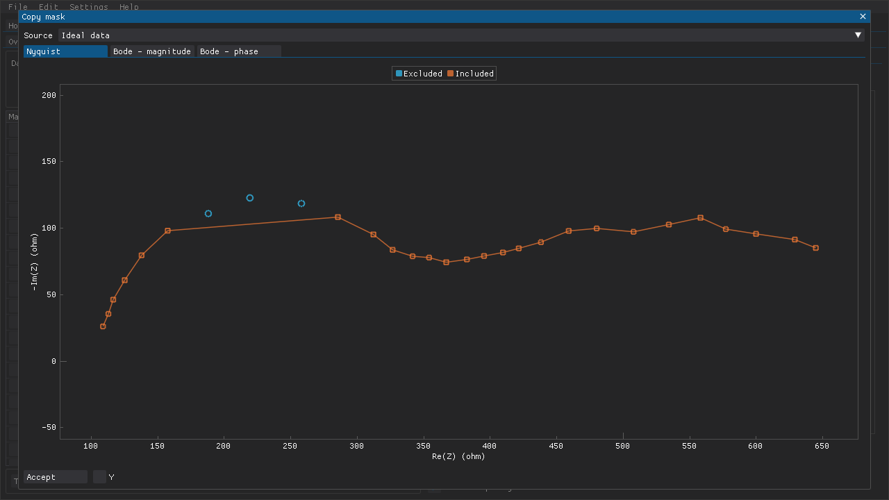
Fig. 5 The Copy mask includes a preview of what the current data set would look like with the mask that was applied to another data set in Fig. 4.

Processing data sets

DearEIS includes a few functions for processing data sets: averaging, interpolation, addition of parallel impedances, and subtraction of impedances. All of these functions are available via the Process button that can be found above the table of data points (Fig. 3). The results of these functions are added to the project as a new data set (i.e., without getting rid of the original data set).

Averaging

The averaging feature can be used to obtain a less noisy spectrum by averaging multiple measurements (Fig. 6). This can be useful in cases where the noise cannot be reduced by adjusting some aspect of the experimental setup (e.g., by improving the shielding). Only data sets with the same frequencies can be averaged.

Note

Make sure that the measurements differ due to random noise rather than, e.g., drift before using this feature.

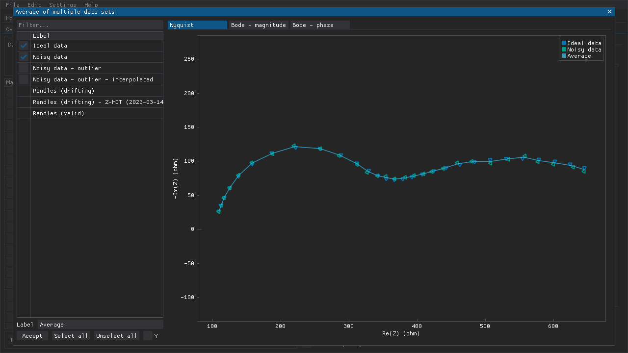
Fig. 6 Two data sets have been chosen (markers) and an average data set has been generated (line). The other data sets do not have the same frequencies as the two chosen data sets and thus cannot be selected while at least one of those two data sets is selected.

Interpolation

The interpolation feature can be used to replace an outlier rather than simply omitting it (Fig. 7). Some specific methods of analysis may be sensitive to the spacing of data points, which is why interpolation may be preferred over omission. The data set is smoothed using LOWESS and interpolated using an Akima spline while ignoring any masked points. Individual data points can then be replaced with a point on this spline by ticking the checkbox next to that data point. Alternatively, if the smoothing and interpolation cannot provide a reasonable result, then values for the real and/or imaginary part of the data point can be inputted directly.

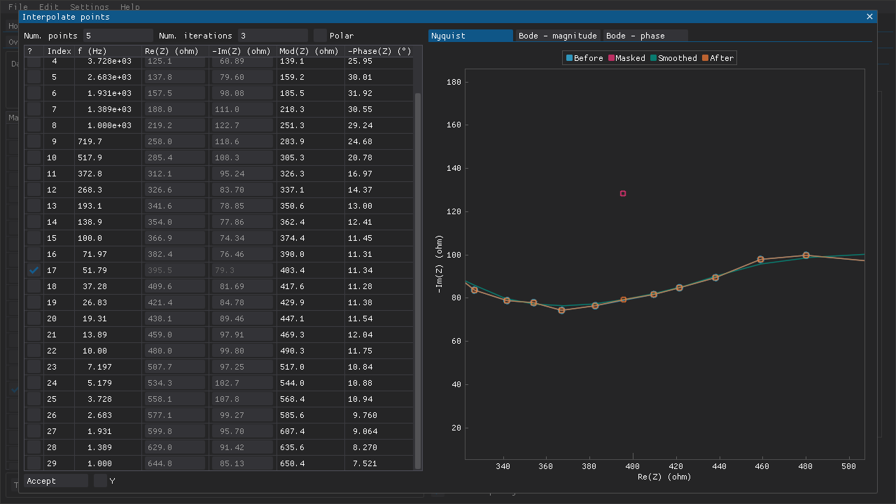
Fig. 7 The outlier (red marker), which was masked in Fig. 3, has been replaced with a value (orange marker) along the interpolated spline (green line).

Adding parallel impedances

Impedance data that include negative differential resistances cannot be validated directly using the included implementations of linear Kramers-Kronig tests. Kramers-Kronig tests can be performed on such data either after transforming it into admittance data (not currently supported) or after adding a suitable parallel resistance to the impedance data. The addition of a parallel resistance does not affect the Kramers-Kronig compliance of the data.

(Source code)

The magnitude of the parallel resistance to add depends on the original impedance data. In the example below (Fig. 8), a resistance of 30 \(\Omega\) was chosen since the absolute value of the real impedance at the lowest frequency was approximately 50 \(\Omega\) (i.e., the point near the x-axis on the left-hand side).

Note

Equivalent circuits can be fitted to the original impedance data that include negative differential resistances provided that negative resistances are allowed (i.e., the lower limits of resistances are disabled or modified prior to fitting).

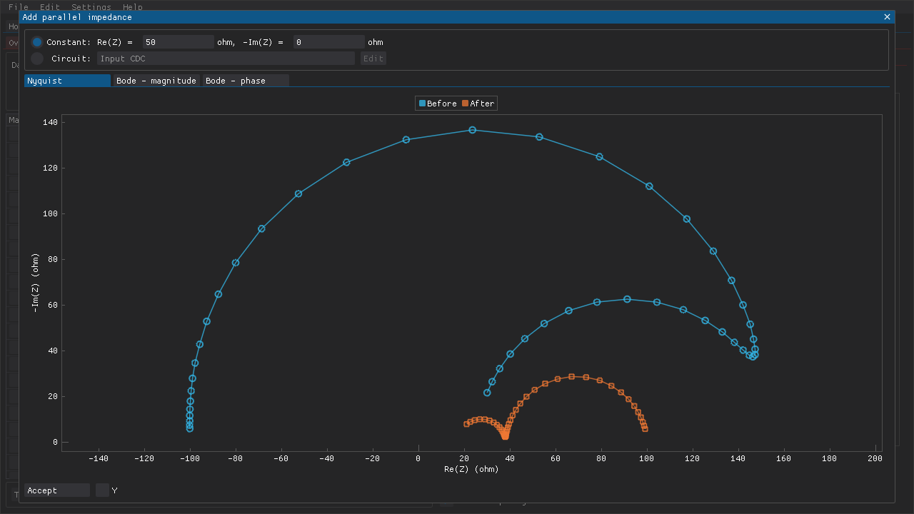
Fig. 8 An impedance spectrum that includes a negative differential resistance was generated for this example (marked here as Before). Performing Kramers-Kronig tests using the implementations included in DearEIS on this impedance data would incorrectly indicate non-compliance even for compliant impedance data. Adding a parallel resistance of 30 \(\Omega\) produces impedance data (marked here as After) that can be validated. The added parallel resistance is always Kramers-Kronig compliant, which means that the compliance of the resulting circuit and its impedance data depends on the compliance of the original data.

Subtracting impedances

The recorded impedances can also be corrected by subtracting one of the following (Fig. 9):

• a fixed impedance

• a circuit

• a fitted circuit

• another data set

This feature can be used to, e.g., correct for some aspect of a measurement setup that is independent of the sample itself.

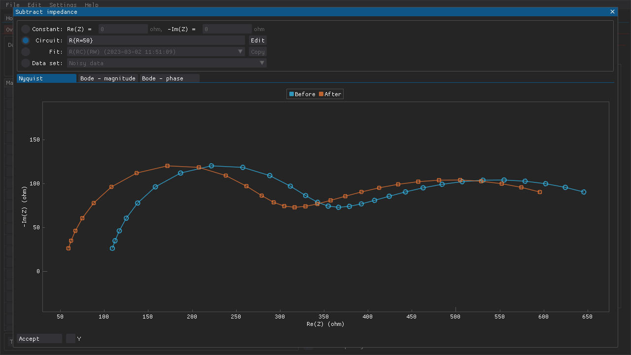
Fig. 9 A resistance of 100 \(\Omega\) is subtracted from a data set.